A research programme · Elies Lucio & Hugues Pouget
Integral Economics
How does the financing of a single venture connect to investment across countries?
Das Kapital: Investment Strikes Back · Elies Lucio & Hugues Pouget
With Hugues Pouget, I study how decisions within a venture connect to markets and the wider economy. What investors know affects what they can fund. Financing then changes ownership and investment, and the resulting financial claims enter household portfolios. Following these links together helps us understand how investment conditions are transmitted across firms and countries.
The explanations introduce each question before the formal results and proofs. In the technical text, GP means the managing partner and LP means an outside investor.
How the programme fits together
The programme connects three levels: individual ventures, meetings between ventures and investors, and the wider economy. The five results below establish parts of this framework under stated assumptions. They cover contracts, risk and financing, successive funding rounds, the allocation of capital and the role of information in an economy where prices adjust.
Micro → MezzoBeliefs, contracts and financing payoffs
Mezzo → MicroMeeting prospects and continuation values
Mezzo → MacroFirm and ownership distributions, cash flows
Macro → MezzoRisk-adjusted returns and aggregate capital
Macro → MicroHousehold state prices
Three levels, linked in both directions. The arrows show how information, financing, ownership and prices connect individual decisions to the wider economy. Select a level to read its research question.
Micro
Information, incentives and financing
What can a venture promise today, and what must its owners retain to invest tomorrow? This level studies how private information, effort, available cash and ownership shape financing terms. Contracts must cover actual payments and make it unattractive to depart from the agreed financial choices. One result replaces a complex payment contract with a finite set of possible payments while preserving its incentives. Another follows two funding rounds and shows how future investment gains can already affect the first financing price.
Mezzo
Ventures and investors
How do ventures and investors find one another? This level connects entrepreneurs’ applications to investors’ offers and the number of ventures they can fund. Better terms may attract more applicants, but an additional offer does not by itself create funds or capacity. The model solves how offers and entry respond to these constraints. It then passes the resulting distribution of funded ventures, ownership and cash flows to the economy-wide analysis.
Macro
Portfolios, prices and the wider economy
How do venture financing and ownership shape international portfolios and returns? This level values cash flows using household state prices: the value placed on a payment in each possible economic situation. Those prices also influence individual financing choices. One result shows why the safe interest rate alone cannot capture this variation. Another studies how new information changes financing after prices adjust, and how the trade balance can change even when net foreign assets remain the same in every economic state.
What these results help us understand
These results trace a path from individual financing contracts to the allocation of capital and international accounts. Each applies to a specified set of institutions and assumptions. Together, they help identify what must be connected to understand investment over the lives of ventures and funds. Bringing these parts into a broader framework is continuing work.
Finite contracts that preserve incentives and funding
Complex payment lotteries can be replaced by a small weighted set without changing the financing or the manager’s privately optimized choices.
Formal result
Consider the specified capped venture-finance institution: a single pooled certificate before effort, payment marks revealed after effort, a committed dealer quote based on actual effort mixing, and a funded mandatory access payment. Service payments are bounded by the venture’s output; purchased financial wealth is capped at four. Successor values are the actual funded-access, registry and posting values.
Every feasible assessment has an equivalent representation on at most eleven joint outcomes across success, failure and nonfinancing. The success-conditional service law has at most nine outcomes. The representation preserves the current funding requirement, both privately optimized financial values, the actual effort mixture, dealer participation and GP utility.
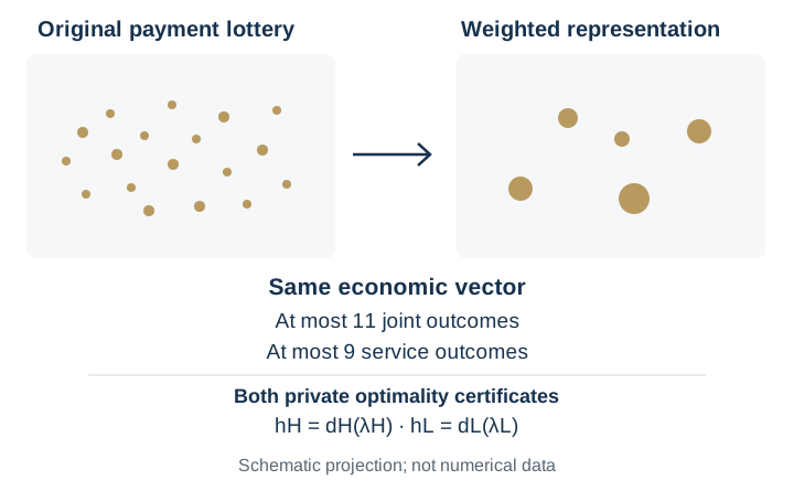
k nonempty branches: at most k + 8 joint outcomes; with k = 3, at most 11. Service outcomes: at most 9.
Illustration
Schematic projection of a higher-dimensional moment vector. The smaller weighted set preserves ten quantities, including both private optimality certificates; the geometry and dot sizes are illustrative, not estimated data.
How the result works
Start with any feasible contract, including its possibly continuous payment lottery. Hold the quote, effort mixture, cash and mandatory access payment fixed. For each effort choice, solve the manager’s entire permitted private financial problem. An attained dual bound certifies that the selected portfolio really is optimal.
Place the two effort-contingent portfolios over the same service draw. This is a way to describe both possible choices together: the manager buys only the portfolio associated with the effort actually chosen. Record a finite vector containing branch probabilities, service cost, premiums, achieved future values, both optimality bounds and the dealer’s profit.
Classical Carathéodory geometry replaces the average of this vector by a weighted combination of finitely many possible outcomes. With three branches, ten coordinates require at most eleven points. At least one point belongs to each nonservice branch, leaving at most nine service-payment points.
The decisive step is preserving the bounds as well as the achieved values. After compression, each selected portfolio still reaches its upper bound, so a newly attractive private deviation cannot appear. Funding, dealer participation and effort choice therefore survive together. The number of possible payments shrinks while the economically relevant assessment remains intact.
Why the safe interest rate cannot summarize financing conditions
The cost of rewarding effort across states changes how much a venture can invest, even at the same safe return.
Formal result
Consider two equally likely aggregate states, linear terminal GP utility, success probabilities p = 4/5 with effort and p₀ = 2/5 without effort, success output 3D and low-effort private benefit (2/5)D. The GP has wealth 1/10 and investment capacity 1; high effort is selected at incentive indifference.
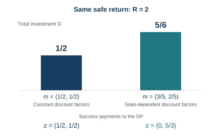
At household discount factors m = (1/2, 1/2), optimal total investment and GP value are (D*, J*) = (1/2, 2/5). At m = (3/5, 2/5), they are (5/6, 2/3), although R = 1/E[m] = 2 in both environments. These are conditional-price optima over both effort choices. Outside LP capital is respectively 2/5 and 11/15.
R = 2 in both cases · D*: 1/2 → 5/6 · J*: 2/5 → 2/3
Illustration
Exact conditional comparison at wealth 1/10. Bars show total investment D; GP contribution is 1/10 in both cases. Payments shown are conditional on success.
How the result works
Start with the compensation needed to make effort worthwhile. In this benchmark, high effort requires the sum of success-contingent payments across the two states to be at least twice investment. Those payments reward the manager, but they also reduce the output that can be pledged to investors.
With constant discount factors, investors put the same price on a unit of compensation in either state. The incentive requirement therefore imposes a fixed limit on pledgeable revenue. Combining that limit with the manager’s wealth of one tenth gives a maximum investment scale of one half.
With state-dependent discount factors, compensation in the second state costs investors less. Put the incentive payment there: the contract with scale five sixths, contribution one tenth and success payments (0, 5/3) satisfies both incentives and investor participation. A bound derived from these same constraints proves that no other high-effort contract yields more.
Finally, compare complete alternatives. Under low effort, output plus the private benefit cannot cover a sufficiently attractive investor payment while improving on saving. This closes the global comparison. The safe return records the average discount factor; it loses the relative prices that determine where incentive compensation is cheapest.
Two financing rounds, one company, one equilibrium
Future investment changes today’s financing terms because the same owners carry their claims into the next round.
Formal result
In the specified two-stage financing game, a privately informed manager can test, delay, negotiate bridges or raise equity. Initial low-type output exceeds the first investment cost; the incumbent cannot finance the cash shortfall alone, two outsiders can underwrite it, and a distinct financier has its own cash K for a deterministic second investment paying Z > K.
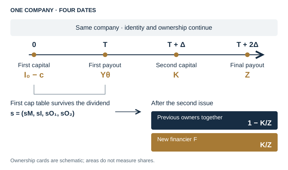
For every primitive vector in the note’s stated domain, an explicitly constructed full-history weak perfect Bayesian equilibrium gives the same surviving company two positive settled primary financings with probability one: I₀ − c at date 0 and K at T + Δ. The first issue pools immediately. Its valuation includes the second investment’s surplus Z − K; the first dividend preserves shares, and the second issue sells fraction K/Z. Here I₀ is the first input cost, c initial company cash, T the first payout date and Δ the time between subsequent financing and payout dates.
Vθ = Yθ + Z − K; λ₂ = K/Z; old owners retain 1 − K/Z; P(two positive financings of the same company) = 1.
Illustration
The same company receives I₀ − c at 0 and K at T + Δ. First dividends use the first cap table; surviving shares are diluted only when the second issue settles. Ownership cards are schematic, not proportional areas.
How the result works
Start at the second investment. A distinct financier already holds the required cash K. Because the project pays a known Z greater than K, selling K/Z of the company exactly repays that financier. The manager chooses this smallest funded fraction, and all surviving owners together keep the surplus Z − K. Funding and consent at equality are part of the equilibrium construction.
Carry that ownership value back to the first round. A first-round share receives both its fraction of Yθ and its fraction of the later surplus. Investors therefore value Vθ = Yθ + Z − K. The incumbent’s private signal changes its contribution, so the pooling price accounts for the capital that the outside underwriters actually supply in each signal state.
Next check the alternatives throughout the game. The assessment specifies financing responses and supported beliefs after every legal history. Away from the initial pool, testing uses company cash and the fixed incumbent policy offers no bridge. A pathwise payoff bound makes immediate financing optimal; any bridge acceptable to the manager cannot improve the incumbent’s payoff. All proposal, contribution and consent alternatives remain available.
Finally join both stages. Even after an earlier deviation changes the company’s history, the second-round payoff bound still applies to its actual surviving shares. Keeping that changed history while replacing only the later strategy proves that no complete two-stage plan improves on the construction. The resulting single equilibrium law finances the same company twice.
How financial contracts direct capital toward entrepreneurs
A funded offer determines an applicant queue; genuine venue capacity turns that queue into investable matches.
Formal result
In the conserved-capacity routing institution, private clues arrive after applications. Suppose precommitted and fully funded menus implement every matched rent split (r, W − r), where W > 0 is total matched surplus. A slot has venue capacity ℓ > 0, c = χℓ/(1 + ℓ), and applicants obtain gross utility u.
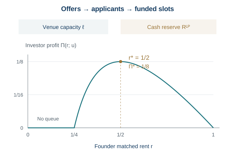
For 0 < u < cW/ℓ, the unique effective rent maximizing Π(r;u) = (c − ℓu/r)₊(W − r) is r*(u) = √(ℓuW/c); offers with no queue earn zero, including r = 0. If founder and investor masses A,F are positive and their continuous cost distributions G,J vanish at zero and are positive at every positive argument, A G(u) = F J(Π*(u))q*(u) has exactly one positive solution. This identifies effective offers and entry. Here q*(u) = √(cℓW/u) − ℓ is the applicant queue per funded slot.
r*(u) = √(ℓuW/c) · Π*(u) = (√(cW) − √(ℓu))²
Illustration
Exact normalized example: ℓ = χ = W = 1, c = 1/2 and u = 1/8. The optimal offer is r* = 1/2, with queue q* = 1 and profit Π* = 1/8. Matching capacity and financial reserves are separate inputs. The proof note also supplies an exact interior-entry example.
How the result works
First establish what a matched contract can distribute. Consolidating real payments and the LP’s funded commitment bounds founder and financier rewards by the available surplus W. An insured information menu attains each division of that surplus, including compensation when tests fail. Promised utility is therefore backed by actual funds.
Next translate offers into applications. Because private information arrives after routing, all applicants face the same prior. Their indifference condition implies the queue q = (cr/u − ℓ)₊. A more generous founder reward attracts a longer queue and raises the chance that the financier fills its slot. The venue carries physical capacity proportional to its slots; a fresh menu label creates neither that capacity nor cash.
The financier balances this higher fill rate against a smaller retained surplus. On the positive-queue region, subtracting any offer’s profit from the proposed optimum gives exactly c(r − r*)²/r. This nonnegative squared loss proves a global optimum. Zero-queue offers yield zero and are strictly worse.
Finally, let founders and financiers enter when the relevant reward covers their own nonpecuniary cost. Founder supply rises weakly with application utility, while financed slot demand times queue length falls strictly. Their curves cross once, producing a positive, unique effective entry outcome. Different funded contracts may implement the same rent split.
Information can sustain venture finance across the economy
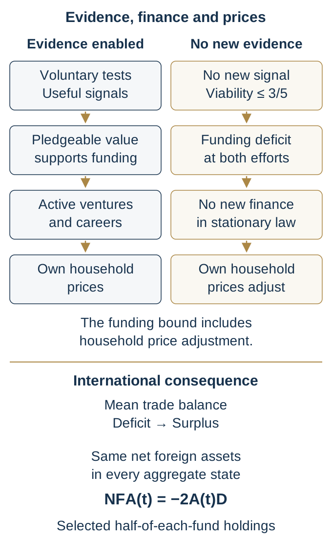
A common stationary economy links evidence to finance and household prices, then shows why removing new evidence can shut investment down even after prices adjust.
Formal result
Consider the specified two-country economy with a small venture sector (GP birth mass 0 < ε ≤ 10⁻⁶ per country), finite GP careers, voluntary evidence, a bounded funded treasury, conserved matching venues and two national funds. GP and retiring-owner cash utility is indexed to productivity; households have log utility. Aggregate productivity A is bounded and positive, the country shock d is bounded by 1/4 and has conditional mean zero, and macro innovations are independent of the physical venture experiments.
For the stated fixed populations, entry costs and small positive country endowment gap D, with μ = E[A] and η = E[Ad] > 0, a common stationary equilibrium has active venture finance and endogenous information. Remove tests and every new viability signal, leaving a viability posterior at most 3/5: every stationary real allocation in the same bounded candidate class is inactive, including candidates that depend on aggregate history. Its equilibrium is constructed with its own household prices and physically funded continuations after off-menu proposals.
Let f > 0 be the active successful-vintage scale and retain the same primitive gap D < 2fη/μ. At the selected half-of-each-fund holdings, the mean trade balance changes from deficit to surplus, while net foreign assets are identical in every aggregate state.
E[TB active] = μD/2 − fη < 0; E[TB inactive] = μD/2 > 0; NFAₜ = −2AₜD in both economies.
Illustration
Mechanism in the specified common economy. The lower panel is a separate international-accounting consequence for the selected half-fund holdings and the stated sign region; no aggregate magnitudes are assigned.
How the result works
Begin with the active economy. Voluntary evidence can raise the viability assessment enough to support an actually funded contract. Optimal young and senior policies generate the venture vintages, payments and household consumption used to determine prices. Founder entry adjusts through an optimal participation probability, so the population and application accounts clear.
Next remove tests and every new viability signal, while allowing communication and financing proposals to remain. Any candidate economy still has bounded household resources because careers, claim maturities and actual collateral calls are finite. Equal household opportunities and log preferences make consumption equal across countries, bounding the prices generated by every candidate allocation.
Those price bounds cannot offset the remaining viability ceiling of three fifths. Under either effort, expected productive value falls short of input cost; the low-effort comparison also includes the private benefit. Adding actual GP, treasury and dealer accounts cancels internal transfers. Private insurance and subsidies across histories cannot create the missing resources, so consuming existing wealth dominates financing.
Zero-wealth newborns therefore refuse, and finite lives remove all old productive vintages from a stationary allocation. Off-menu proposals still receive a real funded continuation before a losing financier rejects them. Basic production then determines the inactive economy’s own prices. Keeping the same country endowment gap preserves statewise net foreign assets, while losing the venture cash-flow term reverses the mean trade balance.